fna.data <- "WisconsinCancer.csv"
wisc.df <- read.csv(fna.data, row.names=1)Class08: Breast Cancer Mini Project
Background
In today’s class we will apply the methods and techniques clustering and PCA to help make sense of a real world breast cancer FNA biopsy data set.
wisc.data <- wisc.df[,-1]
#removes first column from dataset, we don't want to use this for machine learning models, instead will use it later to compare results to the expert diagnosis
diagnosis <- wisc.df$diagnosis
#stores diagnosis column from original dataset in variable "diagnosis"Q1: How many observations are in this dataset?
View(wisc.data)There are 569 observations in this dataset.
Q2: How many of the observations have a malignant diagnosis?
table(wisc.df$diagnosis)
  B   M
357 212 sum(wisc.df$diagnosis == "M")[1] 212table(wisc.df$diagnosis == "M")
FALSE  TRUE
  357   212
There are 212 observations with a malignant diagnosis.
Q3: How many variables/features in the data are suffixed with _mean?
sum(grepl("_mean$", colnames(wisc.data)))[1] 10#either works
length(grep("_mean", colnames(wisc.data)))[1] 10There are 10 observations that are suffixed with “mean”.
Principal Component Analysis
The main function here is prcomp() and we want to make sure we set the optional argument scale=TRUE:
wisc.pr <- prcomp(wisc.data, scale = T)
summary(wisc.pr)
Importance of components:
PC1 PC2 PC3 PC4 PC5 PC6 PC7
Standard deviation 3.6444 2.3857 1.67867 1.40735 1.28403 1.09880 0.82172
Proportion of Variance 0.4427 0.1897 0.09393 0.06602 0.05496 0.04025 0.02251
Cumulative Proportion 0.4427 0.6324 0.72636 0.79239 0.84734 0.88759 0.91010
PC8 PC9 PC10 PC11 PC12 PC13 PC14
Standard deviation 0.69037 0.6457 0.59219 0.5421 0.51104 0.49128 0.39624
Proportion of Variance 0.01589 0.0139 0.01169 0.0098 0.00871 0.00805 0.00523
Cumulative Proportion 0.92598 0.9399 0.95157 0.9614 0.97007 0.97812 0.98335
PC15 PC16 PC17 PC18 PC19 PC20 PC21
Standard deviation 0.30681 0.28260 0.24372 0.22939 0.22244 0.17652 0.1731
Proportion of Variance 0.00314 0.00266 0.00198 0.00175 0.00165 0.00104 0.0010
Cumulative Proportion 0.98649 0.98915 0.99113 0.99288 0.99453 0.99557 0.9966
PC22 PC23 PC24 PC25 PC26 PC27 PC28
Standard deviation 0.16565 0.15602 0.1344 0.12442 0.09043 0.08307 0.03987
Proportion of Variance 0.00091 0.00081 0.0006 0.00052 0.00027 0.00023 0.00005
Cumulative Proportion 0.99749 0.99830 0.9989 0.99942 0.99969 0.99992 0.99997
PC29 PC30
Standard deviation 0.02736 0.01153
Proportion of Variance 0.00002 0.00000
Cumulative Proportion 1.00000 1.00000Q4: What proportion of orginal variance is captured by the first principal component (PC1)?
44.27% of the original variance is captured by PC1.
Q5: How many principal components (PCs) are required to describe at least 70% of the original variance in the data?
It takes 3 PCs to describe at least 70% of the original variance.
Q6: How many principal components are required to describe at least 90% of the original variance in the data?
It takes 7 PCs to describe at least 90% of the original variance.
Interpreting PCA results
Q7: What stands out about this plot? Is it easy or difficult to understand and why?
biplot(wisc.pr)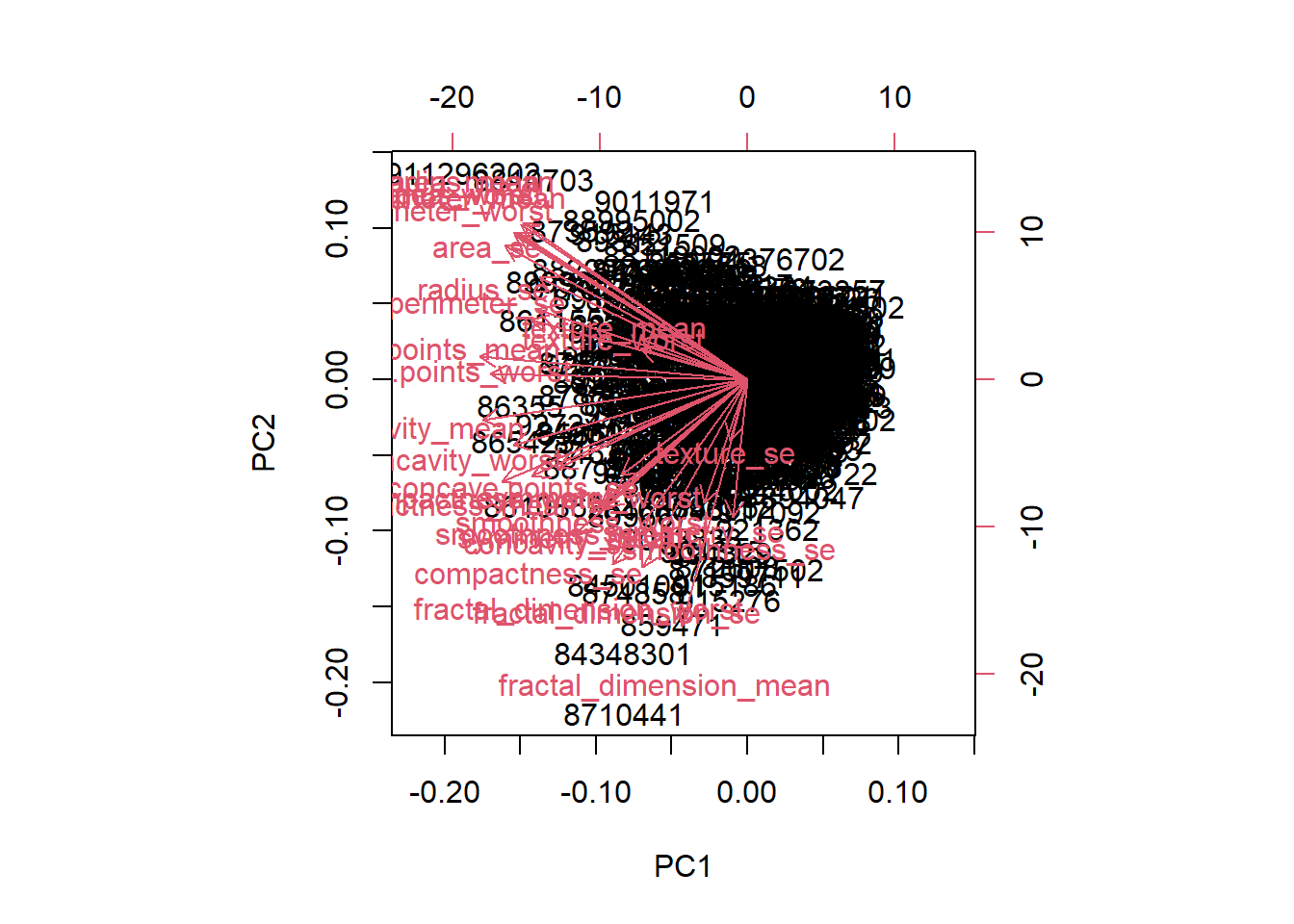
The main thing that stands out about this plot is that all the clusters are all really close together. This density makes the plot difficult to understand as it’s hardd to pick out individual clusters.
Our main PCA “score plot” or “PC plot” of results:
library(ggplot2)ggplot(wisc.pr$x) +
aes(PC1,PC2, col=diagnosis) +
geom_point()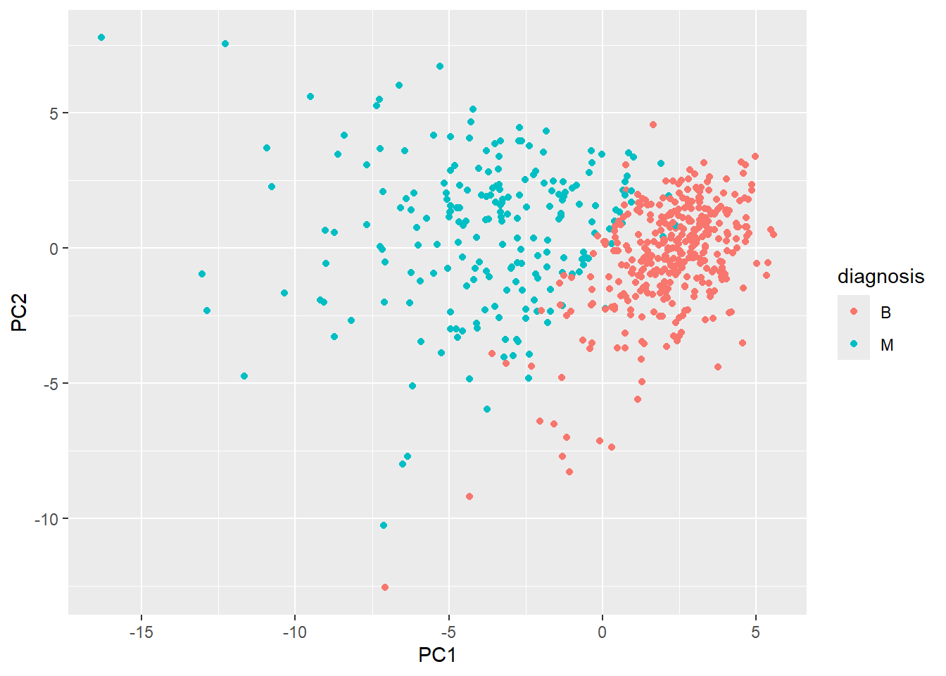
Q8: Generate a similar plot for PCs 1 and 3, what do you notice about these plots?
ggplot(wisc.pr$x) +
  aes(PC1, PC3, col=diagnosis) +
  geom_point()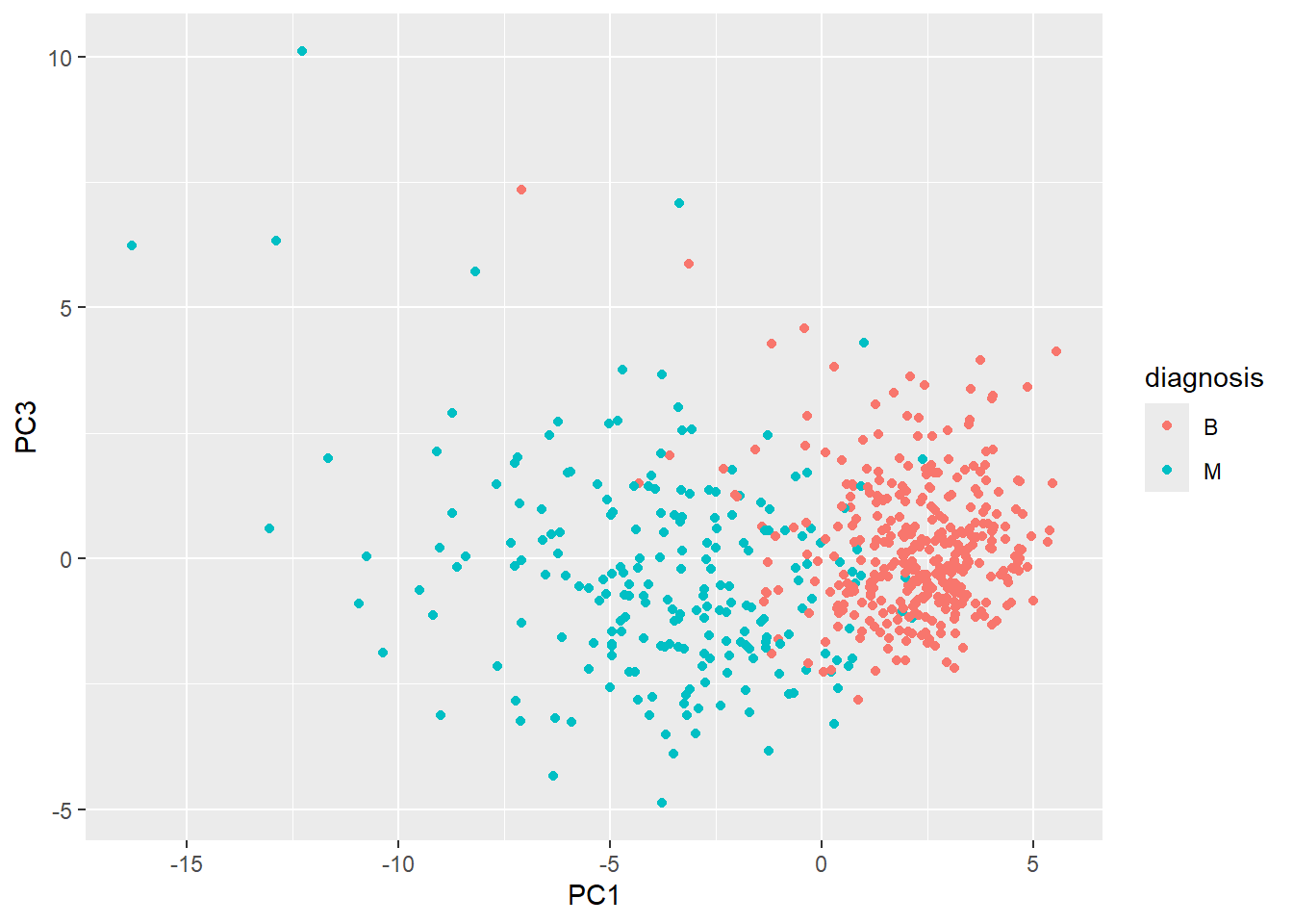
I noticed that in this plot, PC1 appears to be flipped relative to the x-plane and is now upside down compared to the first plot. I notice that in both plots, there’s still a pretty clear distinction between diagnosis “B” and “M”.
Communicating PCA results
Q9: For the first principal component, what is the main component of the loading vector (i.e. wisc.pr$rotation[,1]) for the feature concave.points_mean? This tells us how much this original feature contributes to the first PC. Are there any features with larger contributions than this one?
Hierarchical Clustering
Q10: What is the height at which the clustering model has 4 clusters?
data.scaled <- scale(wisc.data)data.dist <- dist(data.scaled)wisc.hclust <- hclust(data.dist, method = "complete")plot(wisc.hclust)
abline(h = 19, col="red", lty=2)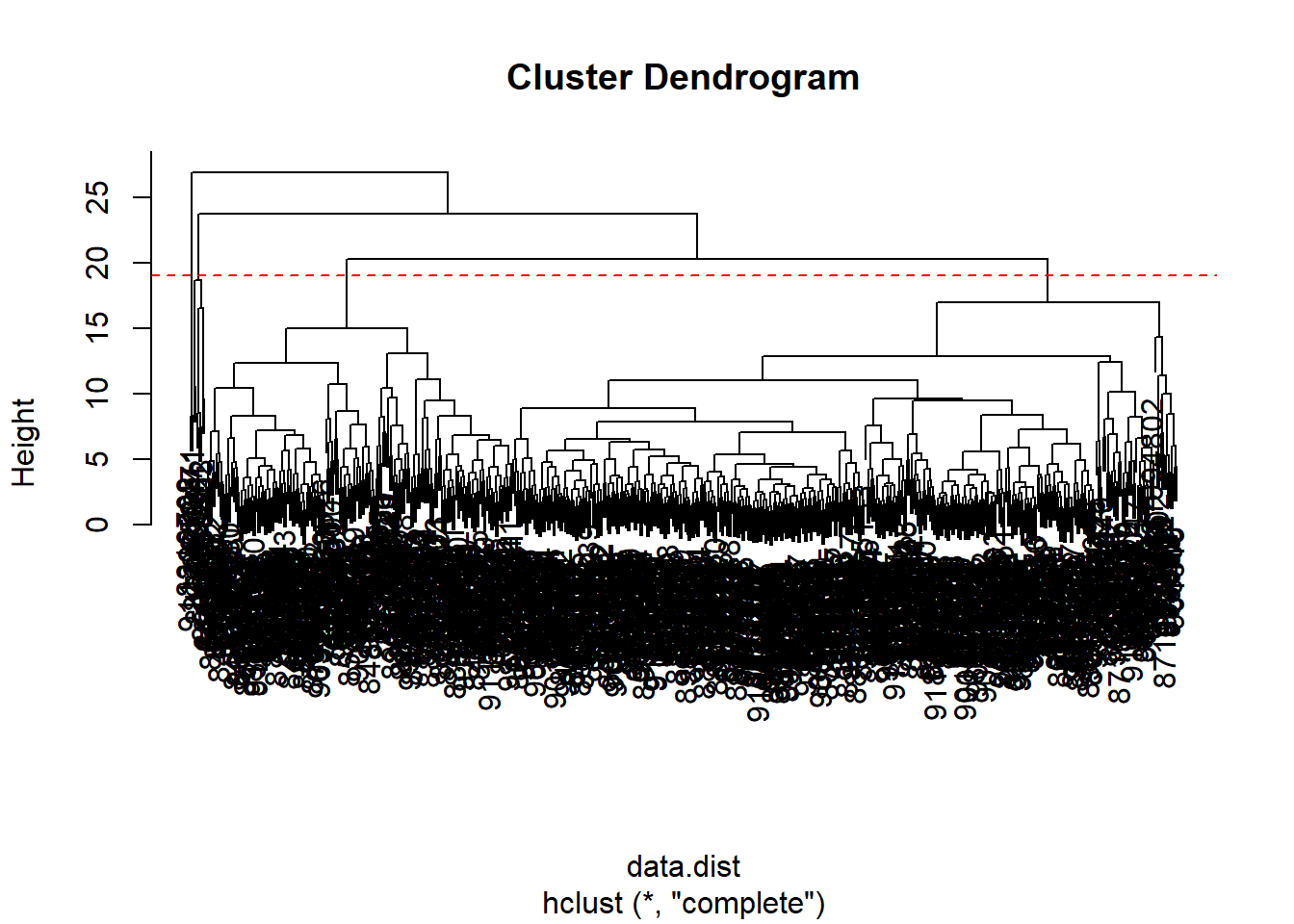
The clustering model has 4 clusters at a height of 19.
wisc.hclust.clusters <- cutree(wisc.hclust,k=4)table(wisc.hclust.clusters, diagnosis) diagnosis
wisc.hclust.clusters B M
1 12 165
2 2 5
3 343 40
4 0 2table(wisc.hclust.clusters)wisc.hclust.clusters
1 2 3 4
177 7 383 2 Combining Methods
Here we will take our PCA resuluts and use those an input for clustering. In other words our wisc.pr$x scores that we plotted above (the main output from PCA - how the data lie on our new principal component axis/variables) and use a subset of the PCs that capture the most variance as input for hclust().
pc.dist <- dist(wisc.pr$x[,1:3])
wisc.pr.hclust <- hclust(pc.dist, method = "ward.D2")
plot(wisc.pr.hclust)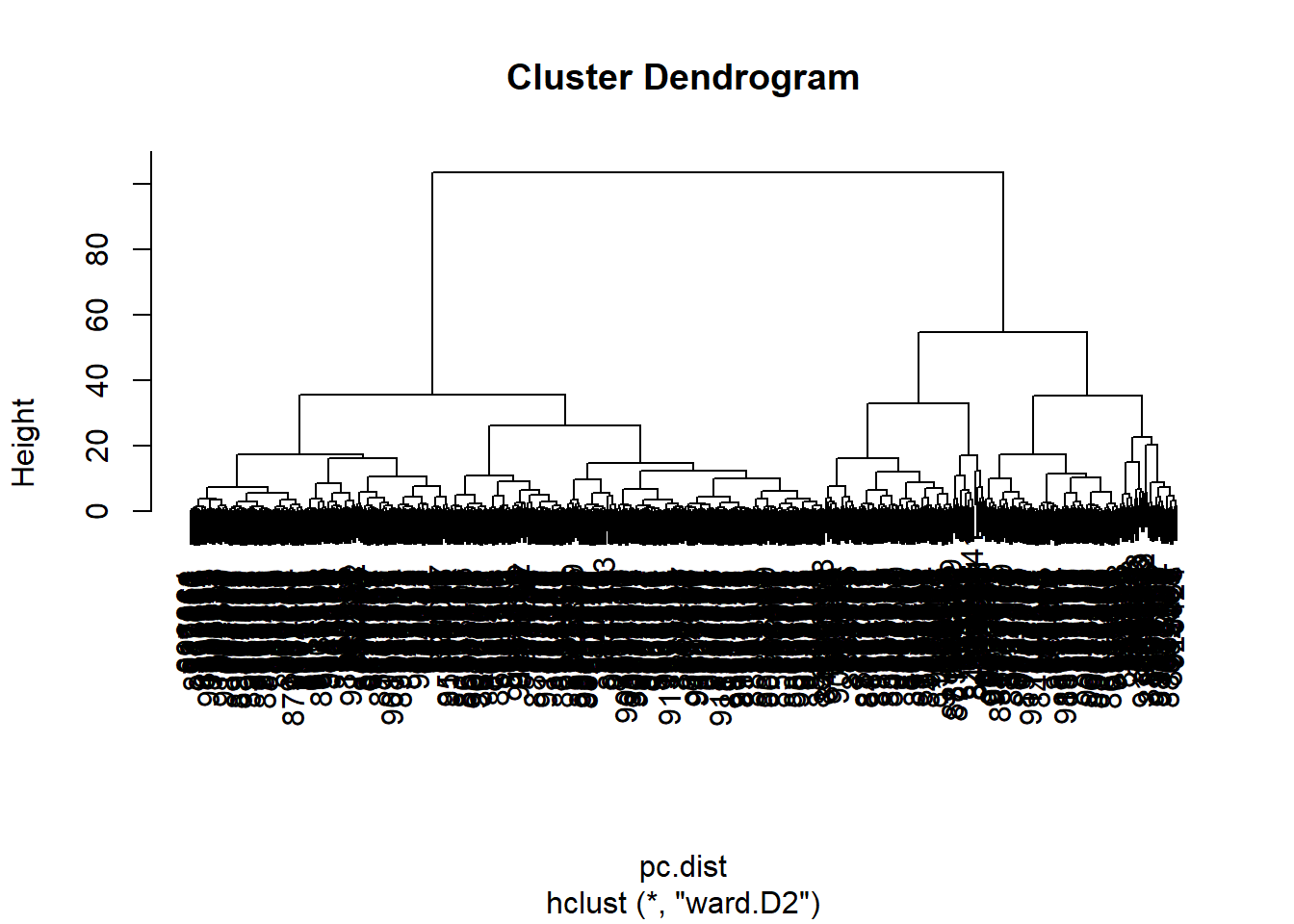
Cut the dendrogram/tree into two main groups/clusters:
grps <- cutree(wisc.pr.hclust, k=2)
table(grps)
grps
1 2
203 366 table(grps, diagnosis) diagnosis
grps B M
1 24 179
2 333 33I want to know how clustering in grps with values of 1 or 2 correspond to the expert diagnosis
table(grps, diagnosis) diagnosis
grps B M
1 24 179
2 333 33My clustering groups 1 are mostly “M” diagnosis (179) and my clustering group 2 are mostly “B” diagnosis (333)
24 FP 179 TP 333 TN 33 FN
Prediction
#url <- "new_samples.csv"
url <- "https://tinyurl.com/new-samples-CSV"
new <- read.csv(url)
npc <- predict(wisc.pr, newdata=new)
npc
PC1 PC2 PC3 PC4 PC5 PC6 PC7
[1,] 2.576616 -3.135913 1.3990492 -0.7631950 2.781648 -0.8150185 -0.3959098
[2,] -4.754928 -3.009033 -0.1660946 -0.6052952 -1.140698 -1.2189945 0.8193031
PC8 PC9 PC10 PC11 PC12 PC13 PC14
[1,] -0.2307350 0.1029569 -0.9272861 0.3411457 0.375921 0.1610764 1.187882
[2,] -0.3307423 0.5281896 -0.4855301 0.7173233 -1.185917 0.5893856 0.303029
PC15 PC16 PC17 PC18 PC19 PC20
[1,] 0.3216974 -0.1743616 -0.07875393 -0.11207028 -0.08802955 -0.2495216
[2,] 0.1299153 0.1448061 -0.40509706 0.06565549 0.25591230 -0.4289500
PC21 PC22 PC23 PC24 PC25 PC26
[1,] 0.1228233 0.09358453 0.08347651 0.1223396 0.02124121 0.078884581
[2,] -0.1224776 0.01732146 0.06316631 -0.2338618 -0.20755948 -0.009833238
PC27 PC28 PC29 PC30
[1,] 0.220199544 -0.02946023 -0.015620933 0.005269029
[2,] -0.001134152 0.09638361 0.002795349 -0.019015820plot(wisc.pr$x[,1:2], col=grps)
points(npc[,1], npc[,2], col="blue", pch=16, cex=3)
text(npc[,1], npc[,2], c(1,2), col="white")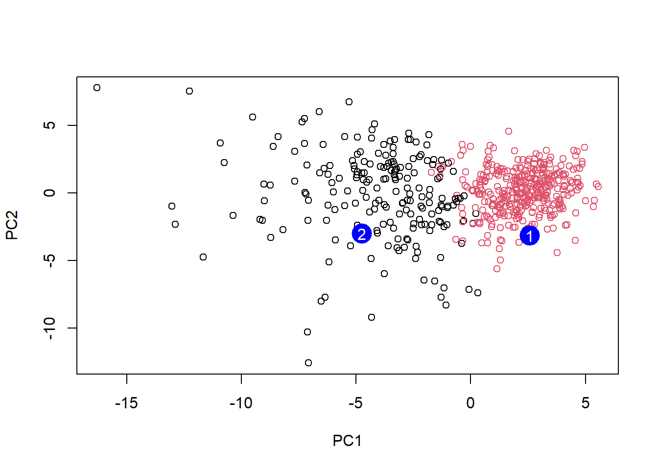
Q16: Which patient should be prioritized for follow up based on the results?
Patient 2 should be prioritized for follow up