Class 12 Pt. 2

Kyle Canturia (A17502778)

Section 1: Identify genetic variants of interest

Downloaded data from Ensembl as a csv file

mxl <- read.csv("373531-SampleGenotypes-Homo_sapiens_Variation_Sample_rs8067378.csv")
head(mxl)

  Sample..Male.Female.Unknown. Genotype..forward.strand. Population.s. Father
1                  NA19648 (F)                       A|A ALL, AMR, MXL      -
2                  NA19649 (M)                       G|G ALL, AMR, MXL      -
3                  NA19651 (F)                       A|A ALL, AMR, MXL      -
4                  NA19652 (M)                       G|G ALL, AMR, MXL      -
5                  NA19654 (F)                       G|G ALL, AMR, MXL      -
6                  NA19655 (M)                       A|G ALL, AMR, MXL      -
  Mother
1      -
2      -
3      -
4      -
5      -
6      -

table(mxl$Genotype..forward.strand.)

A|A A|G G|A G|G 
 22  21  12   9 

GBR dataset

gbr <- read.csv("373522-SampleGenotypes-Homo_sapiens_Variation_Sample_rs8067378.csv")
head(gbr)

  Sample..Male.Female.Unknown. Genotype..forward.strand. Population.s. Father
1                  HG00096 (M)                       A|A ALL, EUR, GBR      -
2                  HG00097 (F)                       G|A ALL, EUR, GBR      -
3                  HG00099 (F)                       G|G ALL, EUR, GBR      -
4                  HG00100 (F)                       A|A ALL, EUR, GBR      -
5                  HG00101 (M)                       A|A ALL, EUR, GBR      -
6                  HG00102 (F)                       A|A ALL, EUR, GBR      -
  Mother
1      -
2      -
3      -
4      -
5      -
6      -

Section 4: Population Scale Analysis

pop <- read.table("rs8067378_ENSG00000172057.6.txt")
head(pop)

   sample geno      exp
1 HG00367  A/G 28.96038
2 NA20768  A/G 20.24449
3 HG00361  A/A 31.32628
4 HG00135  A/A 34.11169
5 NA18870  G/G 18.25141
6 NA11993  A/A 32.89721

#reads dataset and assigns it to a variable

Q13: Read this file into R and determine the sample size for each genotype and their corresponding median expression levels for each of these genotypes.

table(pop$geno)

A/A A/G G/G 
108 233 121 

##only looks at the column "geno" and returns count of how many of each genotype is present

Theres 108 A|A, 233 A|G, and 121 G|G.

library(dplyr) 

Attaching package: 'dplyr'

The following objects are masked from 'package:stats':

    filter, lag

The following objects are masked from 'package:base':

    intersect, setdiff, setequal, union

  pop %>%
  group_by(geno) %>%
  summarize(geno_median = median(exp))

# A tibble: 3 × 2
  geno  geno_median
  <chr>       <dbl>
1 A/A          31.2
2 A/G          25.1
3 G/G          20.1

##uses dplyr tools to first group the samples by genotype, then summarizes the median of each genotype

The median expression levels for A|A, A|G, and G|G are 31.24, 25.06, and 20.07 respectively.

Q14: Generate a boxplot with a box per genotype, what could you infer from the relative expression value between A/A and G/G displayed in this plot? Does the SNP effect the expression of ORMDL3?

library(ggplot2)
ggplot(pop) + 
  aes(geno, exp) +
  geom_boxplot()

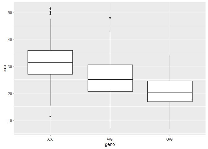
##makes boxplot with geno on the x axis and exp on the y

A|A has the highest expression value while G|G has the lowest, and A|G is in between. From the plot, it’s evident that the SNP is associated with differing expressions of ORMDL3.